Creating heat map report for scroll depth using google sheets google analytics api

Prompted by a tweet

Heat map visualization for scroll depth tracking sorted by top pages for my blog #googleAnalyticsR #measure #rstats cc @bosilytics pic.twitter.com/zpPpgB7Rua

— Ryan Praskievicz (@ryanpraski) February 16, 2017

I set myself a challenge of utilsing Google Sheets and the Google Analytics API to show scroll depth for a group of pages. Here is my step by step guide.

Step 1: Track Scroll

Very obvious, but a must. I do this via Google Tag Manager and some helpful guidance from Andy Gibson. Would also note Luna metrics and Rob Flaherty also have alternatives.

This then fires events into google analytics as follows:

• Event Category: Scroll Depth
• Event Action: Percentage
• Event Label: Baseline, 25%, 50%, 75% or 100%

Step 2: Create a report in google sheets

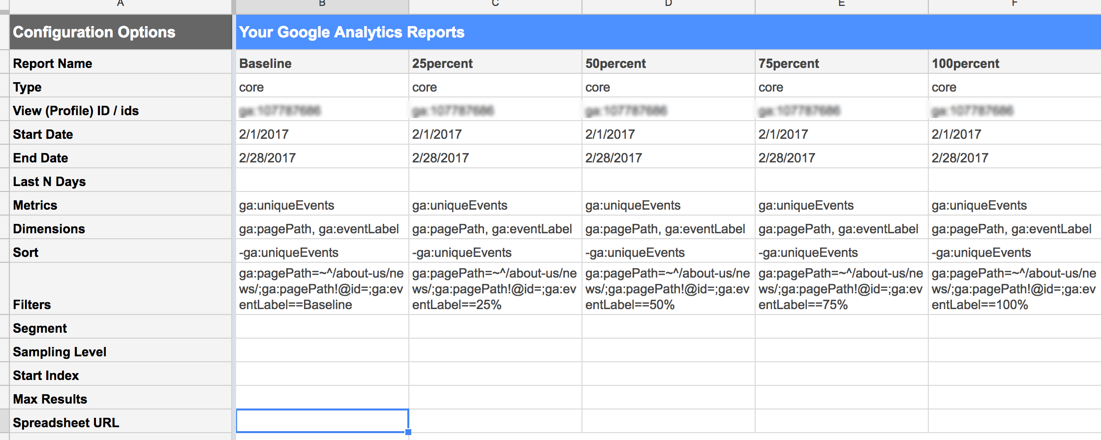
Using the Google Analytics API add on, I have to create a 5 reports for each possible event label. Each consists of the same configuration options, with just a tweak to the filters.

Report Name	Baseline
Type	core
View (Profile) ID / ids	ENTER YOUR ID
Start Date	PICK START DATE
End Date	PICK  END DATE
Last N Days
Metrics	ga:uniqueEvents
Dimensions	ga:pagePath, ga:eventLabel
Sort	-ga:uniqueEvents
Filters	ga:pagePath=~^/about-us/news/;ga:pagePath!@id=;ga:eventLabel==Baseline

You will see I have 2 extra filters. One to show just news pages based on a “regex match” operator (ga:pagePath=~^/about-us/news/) and also a do not show substring operator containing “id=” (ga:pagePath!@id=). This gets me just the right pages to compare. For more info on filter operators check out the google developer site.

Also worth a mention to GDS blog for helpful tips on selecting a date using relative date formulas.

Now repeat this report, changing the last filter and also give it a new report name.

NB I originally used 25%… as a report name, but that played havoc with the tab name in google sheets. So used 25percent…

Run the report

Step 3: Bring the data together

Create a new sheet and give it a meaningful name. Add headings Page path, Baseline, 25%, 50%, 75%, 100%

In cell A2, simply use an array to pull in the baseline data

=ARRAYFORMULA(Baseline!A16:A500)

NB 500 was used to cap the items in my report but you can add more

Repeat for B2

=ARRAYFORMULA(Baseline!C16:C500)

This will pull in the corresponding unique events

For  C2, D2, E2 and F2 you need to use a vlookup to match the url from a2 and pull in the matching unique event.

=iferror(VLOOKUP(A2, '25percent'!A$15:C$500, 3, 0))

=iferror(VLOOKUP(A2, '50percent'!A$15:C$500, 3, 0))

=iferror(VLOOKUP(A2, '75percent'!A$15:C$500, 3, 0))

=iferror(VLOOKUP(A2, '100percent'!A$15:C$500, 3, 0))

NB I wrap the vlookup with an iferror to clear the N/A to a blank.

Select the cells with rules and pull the cells down to fill the rest of the rows.

What you are left with is a table of urls based on diminishing unique events. This you can take to Step4 or if your data is like mine (biased by one page) you can add some more cells that just give you a percentage drop out.

So in columns H-L i recreate the titles (Baseline, 25%, 50%, 75%, 100%) and then do some simple sums in row 2, formatting them to a percentage.

=B2/B2

=C2/B2

=D2/B2

=E2/B2

=F2/B2

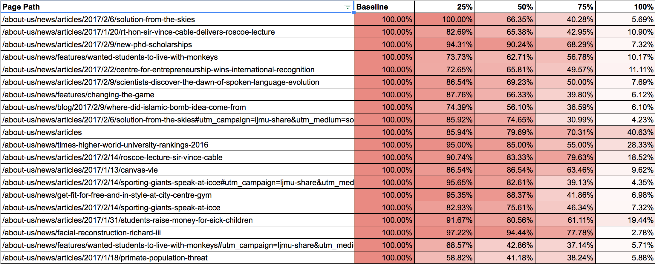
Step 4: Conditional formatting

Google sheets makes this a very simple task. Select the data to format. Go to Format and Conditional Formatting in the menu. A new rule box appears on the right. I chose the 2nd tab “color scale”. Picked the white to red, which gives the smallest value white and the largest red. And click done.

Below are my 2 examples (one just based on unique events, the other on a percentage calculation.

Here is my test google sheet if people want to look.

Notes

Now I release there are more visual heat map tools, which I also advocate. These are great for research workshops or senior stakeholder presentations. There visual, they connect instantly. Please use them.

The reason I have used google sheets is for a different audience. The beauty of google sheets is the fact it relays data both timely (auto schedules) but also in a format that you control (the language, the look…) The audience doesn’t need to understand google analytics or its terminology, they just need to understand your google sheets report.

By providing heat maps in this format for highly valuable pages (news pages, product pages, list pages) you can see instant insight. Now “read” is a strong word, just because someone scrolls does not mean they read content, but knowing that someone scrolled, even past the baseline means someone was vaguely interested.

Now to crank this up a level, and what I do for LJMU is swap the scroll event funnel for engagement funnel.

So rather than the use of a filter per report, I use segments, one for all traffic (baseline), one for no bounce, one for engagement (a collection of various events) and one for the main CTA.

Please let me know your thoughts.